In prediction tasks, given data does not necessary consist of only useful information. The data may contain irrelevant features, which impairs the performance of a predictor due to overfitting. This situation is often the case for medical data. Sometimes, only a few hundreds of samples are available while we have thousands of features. In this case, we have to extract a small subset of effective features to reduce computational costs and overfitting. Random forest is one of the popular predictors due to the robustness. As one of the useful byproducts, random forests are able to estimate how much each feature has an effect on a performance of the forests. Thus, random forests give us one of possible approaches to reduce the number features to use. In this article, we work on a binary classification task of “Dorothea Data Set” from UCI Machine Learning Repository. We show that features selected by random forests are efficient not only for random forests themselves but also for logistic regression.

1. Background¶

Random forests has been introduced by Breiman in the paper in 2001. He proposed collecting many classification and regression trees(CART) and used them to establish better predictors. The key concept of random forests is bagging introduced by Breiman in the paper in 1994. The name comes from the combination of acronym of two words: bootstrap and aggregating. Bagging has been succeeded to improve unstable predictors like neural network and CART. By applying bagging to CART, we obtain the better accuracy tree, random forests. As one of the useful byproducts, we can use random forests to measure importance of each input feature. We explain these concepts in the following order: bootstrap, bagging, and random forests.

1.1. Bootstrap¶

Bootstrap is a general methodology to measure the accuracy of estimations based on resampling, which has been introduced by Efron and Tibshirani in the paper. Since the variance of an estimation is frequently used to measure the accuracy of estimation, bootstrap is practically used to guess the variance of the estimation. Especially, bootstrap gives us a computational approach to analytically intractable cases.

Let's say we have $n$ samples from distribution $F$ and estimate its mean with the unbiased estimator, $$ \bar{x} = \sum_{i=1}^n x_i / n.$$ Let us denote by $\mu_2 (F) = E_F X^2 - (E_F X)^2$ the variance of distribution $F$. We analytically calculate the standard deviation $\sigma(F; N, \bar{x})$ as $$\sigma (F) = [\mu_2 (F) / n]^{1/2},$$ where $\sigma(F) \equiv \sigma(F; n, \bar{x})$. Since $\mu_2 (F) $ is unknown function, we use unbiased estimator $\bar{\mu}_2 = \sum_{i=1}^n (x_i - \bar{x})^2 / (n - 1)$ instead; i.e., we have $$\bar{\sigma} = [\bar{\mu}_2 / n]^{1/2}.$$

There is another way. Let $\hat{F}$ be the empirical distribution; i.e., $\hat{F}$ assigns the probability mass $1/n$ to each data point $x_i$. Then, we obtain $$\bar{\sigma} \equiv \sigma(\hat{F}) = [\mu_2(\hat{F}) / n]^{1/2},$$ where $\mu_2(\hat{F}) = \sum_{i=1}^n (x_i - \bar{x})^2 / n$. This approach is more flexible. In the above mean estimation example, we have to know the analytical expression of unbiased estimation of the variance, which is not often the case for more complex estimations.

To apply the second method to even more complex cases, we introduce the new sampling concept called bootstrap sampling. Let us assume that we estimate $\theta$, which corresponds to $E_F X$ in the previous example. To formalize into the second method, we need to calculate $$E_{\hat{F}} (\hat{{\theta}}(\bf{x}) - E_{\hat{F}} \hat{{\theta}}(\bf{x}))^2,$$ where $\hat{F}$ is the empirical distribution of n data points $\bf{x} = (x_1, x_2, \dots, x_n)$. Since computing all of the case $\hat{{\theta}}(\bf{x})$ is too expensive, we resort to Monte Carlo method; i.e., we take sample mean with B sets of data $\{\bf{x}^b\}_{b=1}^B = \{x_1^b, x_2^b, \dots, x_n^b\}_{b=1}^B$ sampled from empirical distribution $\hat{F}$. Note that all of sets must have exactly n data because the expression of estimation depends on n. This sampling method is called bootstrap sampling. Taking sample mean instead of expectation leads to $$\theta^*(\cdot) = \frac{\sum_{b=1}^B \hat{\theta }(b)}{B}$$ $$\sigma_B = \left(\frac{\sum_{b=1}^B (\hat{\theta}(b) - \theta^*(\cdot) }{B - 1}\right)^{1/2}.$$ $\sigma_B$ can be used to measure the accuracy of the estimation.

For more precise discussion over the accuracy of this method itself, you can check the original paper.

1.2. Bagging¶

Bagging has been introduced by Breiman in the paper. He used bootstrap sampling to improve the accuracy of unstable predictors. The concept is quite simple. Consider a predictor trained by training set $\mathcal{L}$. For each input $x$, prediction can be expressed as $\varphi(x, \mathcal{L})$. For regression case, we can define the aggregated predictor as $$\varphi_A(x) = E_{\mathcal{L}} \varphi(x, \mathcal{L}).$$

For the classification case, the class voted by the most predictors would be the prediction value. That is, each $\varphi(x, \mathcal{L})$ has C dimensional output $\varphi(x, \mathcal{L}) = (\varphi^1(x, \mathcal{L}), \varphi^2(x, \mathcal{L}), \dots, \varphi^C(x, \mathcal{L}))$ and each component corresponds to each class confidence. Then, the aggregated predictor is defined as $$\varphi_A(x) = \underset{1 \leq c \leq C}{max} E_{\mathcal{L}} \varphi^c(x, \mathcal{L}).$$

This aggregation procedure especially increase the accuracy of unstable predictors. Consider the regression case. We have the generalized prediction error in $\varphi (x, \mathcal{L})$ and $\varphi_A(x)$: $$e = E_{\mathcal{L}} E_{y, x} (y - \varphi(x, \mathcal{L}))^2,$$ $$e_A = E_{y, x} (y - \varphi_A(x))^2.$$ Then, we obtain $$e = E_{\mathcal{L}} E_{y, x} y^2 - 2 E_{y, x}y \varphi_A(x) + E_{\mathcal{L}} E_{y, x} \varphi(x, \mathcal{L})^2\\ \geq E_{y, x} (y - \varphi_A(x))^2\\ = e_A,$$ where we use Jensen inequality, $E_{\mathcal{L}}\varphi(x, \mathcal{L})^2 \geq (E_{\mathcal{L}}\varphi(x, \mathcal{L}))^2$. Hence, aggregated predictor has better performance if and only if $E_{\mathcal{L}}\varphi(x, \mathcal{L})^2$ is strictly greater than $(E_{\mathcal{L}}\varphi(x, \mathcal{L}))^2$, which implies that unstable predictors — large variance predictors — will be improved by the aggregation.

In the practical situation, the calculation of $E_{\mathcal{L}} \varphi(x, \mathcal{L})$ is often intractable. Then, we often use $$\varphi_B(x) = \hat{E}_{\mathcal{L}} \varphi(x, \mathcal{L}),$$ where $\hat{E}(\cdot)$ is empirical expectation calculated through bootstrap sampling. Bootstrap sampling gives us some numerical errors between $\varphi_B(x)$ and $\varphi_A(x)$. Therefore, there is cross-over point between instability and stability at which $\varphi_B(x)$ stop improving and does worse. Indeed, there is the example that stability predictor does worse through bagging in the paper.

In classification, a predictor predicts a class label $c \in \{1, 2, \dots, C\}$. The probability of correct classification can be calculated as $$r(\mathcal{L}) = \sum_{c} P(\varphi(x, \mathcal{L}) = c | y = c) P(y = c).$$ We define $Q(c | x) \equiv P_{\mathcal{L}}(\varphi(x, \mathcal{L}) = c)$, where$P_{\mathcal{L}}$ is probability measure of samples $\mathcal{L}$. By taking marginalization over $P_\mathcal{L}$, we have $$r = \sum_{c}E[Q(c | x) | y=c] P(y = c)\\ = \sum_{c} \int Q(c | x) P(y=c|x) P_x(dx).$$

Since the aggregated predictor is equivalent to $\varphi_A(x) = \underset{c}{argmax} Q(c | x)$, we can write down the probability of correct classification of the aggregated predictor as $$r_A = \sum_{c} \int I(\underset{j}{argmax} Q(j | x) = c) P(y=c|x) P_x(dx),$$ where $I(\cdot)$ is the indicator function. Consider a set $D$, $$D = \{x; \underset{c}{argmax} Q(c | x) = \underset{c}{argmax} P(c | x) \}.$$ We can express $r_A$ as $$r_A = \int_D \underset{c}{max}P(y=c|x) P_x(dx) + \sum_{c} \int_{D^c} I(\varphi_A(x) = c) P(y=c|x) P_x(dx).$$

For each predictor, the highest attainable correct prediction is obtained when $P_x(D) = 1$; i.e., we have $$r^* = \int \underset{c}{max}P(y=c|x) P_x(dx).$$ For $x \in D$, $\sum_{c} Q(c | x) P(y = c | x)$ can be less than $\underset{c}{max}P(y=c|x)$. Thus, even if $P_x(D) \simeq 1$, non-aggregated predictor might be far from optimal.

In classification, aggregation actually improves the performance more for the better performance predictor. This can be deduced from the above expression of $r_A$. In order to have the performance close to optimal one $r^*$, we have to assign large probability mass to $D$; i.e., the predictor already have high probability of correct classification. As to the stability of the predictor, the same statement as regression holds for classification.

1.3. Random Forests and Feature Importance¶

Random forest has been introduced by Breiman in the paper . As we discussed previously, bagging improves the accuracy of unstable predictors like neural network and CART. Then, He applied bagging to CART to improve the accuracy.

Concept is quite simple. At every node, we just split data depending on subset of variable. Let's say we have $M$ dimensional input feature. At every node, randomly chosen subset $s$ variables of $M$ variables are used to split data. After established some trees, we mean of outputs of trees for regression, or take vote as to which class will data should be classified for classification.

As one of the useful byproducts of bootstrap sampling, we have unused samples called out-of-bags, which has been discussed in the paper by Breiman. When using bootstrap sampling, we have unsampled data for each set. This comes from the following:

Let $N$ be the number of data. The probability to unsample one of the data $x_i$ is $(1 - \frac{1}{N})^N$. By using the fact that $\underset{n\to \infty}{lim}(1 + \frac{1}{N})^{-N} = \frac{1}{e}$, we can lead to $\underset{N \to \infty}{lim}(1 - \frac{1}{N})^N = \frac{1}{e} \simeq 0.3679$. Thus, for large enough data, almost 37% data will not be sampled. Using these unsampled data, we can improve accuracy of prediction for important some statistical quantities. For example, it is known that training error has downside bias. We can use out-of-bag to have more accurate estimation of generalized error without any additional data. Thus, to evaluate the performance of random forests, we need neither of test data nor additional computational time coming from cross validation.

As another useful byproducts, we have feature importance. This is a quantity to measure the importance of each component of input for prediction. As we mentioned above, the performance of random forest is measured on out-of-bag. The performance should be measured by certain criteria such as Gini index, entropy, and accuracy. Then, we add noise to each variables and see how much the value of the criteria changes. We do this through the following process.

Let us assume that we use $M$ dimensional input feature $\bf{x} = (x_1, x_2, \dots, x_M)$ and $N_T$ trees for estimation.

FOR $i = 1$ to $N_T$

• Generate a tree
• Evaluate performance on out-of-bag

FOR $m = 1$ to $M$

• Collapse $x_m$ by noise
• Evaluate and save the change of the value of the criteria

END FOR

END FOR

• Take mean saved changes (The higher, the more important)

Through this process, we identify which component is significant for prediction. In scikit-learn implementation, normalized criteria are used to evaluate the feature importance; they measure how much noised feature increases the value of criteria in the percentage. Gini impurity and mean squared error used as default for classification and regression respectively.

2. Experiments¶

When developing new drugs, we have to specify which compound of ingredients works on a human body. We here call active or inactive for if compounds are effective or not. Dorothea Data Set contains labels and binary features. Labels indicate if each compound is active(positive) or inactive(negative), and binary features correspond to which ingredients out of 100,000 kinds each compound contains. Dorothea Data Set has 800, 350, and 800 instances for training, validation, and test set respectively. Since labels of test data are not available, we use validation data as test data instead. Hence, we have training input: (800, 100000), test input: (350, 100000), training label: (800, ), and test label: (350, ).

2.1. Fetch data¶

In the repository, labels are expressed as -1 (negative) or +1(positive), and we convert them into 0 (negative) or 1(positive). For binary features, each candidate is recorded as [3, 14, 56, 146, ....., 99953, 99999], where numbers indicate which features exist. We convert features into binary data; e.g., [0, 0, 1, 0, ....., 1, 0].

2.2. Feature Importance¶

Let's estimate importance of feature!

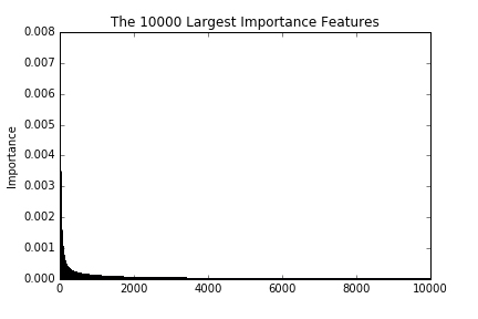
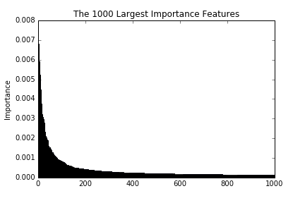
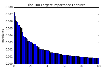
These figures are the largest 100, 1000, and 10000 importance of features. As we see in the figures, the importance decreases drastically till reaching around 100. This implies that a prediction with the top 100 importance features is able to attain good enough performances.

2.3. Performance¶

Let’s see the effectiveness in numerical experiments. Less than 10% instances of given data contains are positive. That is, the class distribution is skewed. In this situation, usual accuracy does not work. For instance, consider the case where there are 99% negative and 1% positive instances. Even a predictor that always returns negative achieves 99% accuracy. On the other hand, a predictor that predict classify negative instances with 98% correctly and positive instances with 99% correctly achieves only 98.01% accuracy as a whole. Does that mean the former predict is better than the latter one? Not necessary! Sometimes, detecting the class occupying small portion of data is more important; e.g., cancer diagnosis.

When working on binary classification task, we usually first have real value outputs from a predictor and classify instances over a certain threshold into positive. Mostly, the outputs are restricted to [0, 1] and the threshold is set as 0.5. This setting may work when class is equivalently distributed; i.e., positive 50% and negative 50%. Skewed class distribution, however, cause too little detecting the smaller occupation side. This comes from the learning architecture. In most cases, we use a non skewed cost function like binary cross entropy in the learning stage, which makes outputs incline to the negative side.To avoid this, we have to set threshold as a hyper parameter. There is a measure taking this problem into consideration called receiver operating characteristic(ROC). Taking TPR and FPR as y-axis and axis respectively, the measure visualize the performance of a predictor with plot along with various thresholds. This plot is called ROC Curve. The area under this curve in the graph is often used as a measure of the performance of predictors, which is called the area under an ROC Curve (AUC). We use AUC to evaluate the performance.

We test the performance of random forests and logistic regression. As a benchmark, we use a predictor with randomly chosen input features.

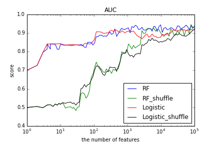
Results labeled “_shuffle” correspond to AUC scores of predictors with randomly chosen input features. Logistic regression with selected features almost reached the peak around 100 features as well as random forests. With more features, logistic regression had rather worse performance. Compared to the scores of “_shuffle”, we saw that predictors with selected features had significantly better performance with small number of features.

3. Discussion¶

We worked on feature selection with random forests for “Dorothea Data Set”, and evaluated the effectiveness with random forest itself and logistic regression. Only 100 out of 100000 features could reach the almost the best performance for both algorithms. Especially, logistic regression had better performance with small number of features through avoiding overfitting coming from the high dimensional input. This result imply the possibility that the importance of feature could be applied to other algorithms with high dimensional input.