Data Explore and Visualization
Data exploration is important. Before jumping into analysis, you will get some intuition as to how to use data and establish more sophisticated modeling. In some cases, how to use data improve even models robust to high dimensional input like Deep Learning. In this article, we work on data exploration and visualization for the house price data from a kaggle competition. This gives effective features selection, which has better performance than random feature selection.
Data Exploration and Visualization
House prices are determined through various factors such as location, quality, and size. Before jumping into analysis, we explore given data. Our data exploration process is divided into a few steps:
Understand the Problem: Figure out characteristics of given data and the meaning of each feature
Univariate Study: Focus on understanding the characteristic of target value, 'SalePrice'.
Multivariate Study: Explore the relations among input features and target value.
Feature Selection: Determine which features have to be employed as input.
1. Understand the Problem
In this section, we look into basic information of given data. We have two kinds of data: train data and test data. Train data and test data have 1460 and 1459 candidates respectively. While both have 80 input features, target value, 'SalePrice', is given to train data additionally; i.e., shapes of train and test data are (1460, 81) and (1459, 80) respectively.
%matplotlib inline
import numpy as np
import pandas as pd
import matplotlib.pyplot as plt
import seaborn as sns
df_train = pd.read_csv('train.csv')
First, we consider classifying input features into a few categories. In given data, we have the following features:
'Id', 'MSSubClass', 'MSZoning', 'LotFrontage', 'LotArea', 'Street', 'Alley', 'LotShape', 'LandContour', 'Utilities', 'LotConfig', 'LandSlope', 'Neighborhood', 'Condition1', 'Condition2', 'BldgType', 'HouseStyle', 'OverallQual', 'OverallCond', 'YearBuilt', 'YearRemodAdd', 'RoofStyle', 'RoofMatl', 'Exterior1st', 'Exterior2nd', 'MasVnrType', 'MasVnrArea', 'ExterQual', 'ExterCond', 'Foundation', 'BsmtQual', 'BsmtCond', 'BsmtExposure', 'BsmtFinType1', 'BsmtFinSF1', 'BsmtFinType2', 'BsmtFinSF2', 'BsmtUnfSF', 'TotalBsmtSF', 'Heating', 'HeatingQC', 'CentralAir', 'Electrical', '1stFlrSF', '2ndFlrSF', 'LowQualFinSF', 'GrLivArea', 'BsmtFullBath', 'BsmtHalfBath', 'FullBath', 'HalfBath', 'BedroomAbvGr', 'KitchenAbvGr', 'KitchenQual', 'TotRmsAbvGrd', 'Functional', 'Fireplaces', 'FireplaceQu', 'GarageType', 'GarageYrBlt', 'GarageFinish', 'GarageCars', 'GarageArea', 'GarageQual', 'GarageCond', 'PavedDrive', 'WoodDeckSF', 'OpenPorchSF', 'EnclosedPorch', '3SsnPorch', 'ScreenPorch', 'PoolArea', 'PoolQC', 'Fence', 'MiscFeature', 'MiscVal', 'MoSold', 'YrSold', 'SaleType', 'SaleCondition'
When considering purchasing a house, what comes into your mind first is the location. Convenience of access to your workplace or school is one of the most important factors. Next, we may consider the size. If you have your family in your house, you may need larger house. Finally, we consider the quality. The higher quality, the more expensive. Considering above, we divide input features into three categories: location, size, and quality.
Location:
'Neighborhood', 'Condition1', 'Condition2'
Size:
'LotFrontage', 'LotArea', 'MasVnrArea', 'BsmtUnfSF', 'TotalBsmtSF',
'BsmtFinSF1', 'BsmtFinSF2', '1stFlrSF', '2ndFlrSF', 'LowQualFinSF',
'GrLivArea', 'GarageCars', 'GarageArea', 'WoodDeckSF', 'OpenPorchSF',
'EnclosedPorch', '3SsnPorch', 'ScreenPorch', 'PoolArea'
Quality:
'MSSubClass', 'MSZoning', 'Street', 'Alley', 'LotShape', 'LandContour',
'Utilities', 'LotConfig', 'LandSlope',  'BldgType', 'HouseStyle',
'OverallQual', 'OverallCond', 'YearBuilt', 'YearRemodAdd', 'RoofStyle',
'RoofMatl', 'Exterior1st', 'Exterior2nd', 'MasVnrType', 'ExterQual',
'ExterCond', 'Foundation', 'BsmtQual', 'BsmtCond', 'BsmtExposure',
'BsmtFinType1', 'BsmtFinType2', 'Heating', 'HeatingQC', 'CentralAir',
'Electrical',  'BsmtFullBath', 'BsmtHalfBath', 'FullBath', 'HalfBath',
'BedroomAbvGr', 'KitchenAbvGr', 'KitchenQual', 'TotRmsAbvGrd',
'Functional', 'Fireplaces', 'FireplaceQu', 'GarageType', 'GarageYrBlt',
'GarageFinish', 'GarageQual', 'GarageCond', 'PavedDrive', 'PoolQC',
'Fence', 'MiscFeature', 'MiscVal', 'MoSold', 'YrSold', 'SaleType',
'SaleCondition', 'SalePrice'
Other than above categorization, we have to consider types of data. Given data has two kinds: numerical and categorical.
numerical = [x for x in df_train.columns if df_train.dtypes[x]!='object']
# index is used instead of Id to identify an element
numerical.remove('Id')
numerical.remove('SalePrice')

categorical = [x for x in df_train.columns if df_train.dtypes[x]=='object']
Numerical:
'MSSubClass', 'MSZoning', 'LotFrontage', 'LotArea', 'Street', 'Alley', 'LotShape', 'LandContour', 'Utilities', 'LotConfig', 'LandSlope', 'Neighborhood', 'Condition1', 'Condition2', 'BldgType', 'HouseStyle', 'OverallQual', 'OverallCond', 'YearBuilt', 'YearRemodAdd', 'RoofStyle', 'RoofMatl', 'Exterior1st', 'Exterior2nd', 'MasVnrType', 'MasVnrArea', 'ExterQual', 'ExterCond', 'Foundation', 'BsmtQual', 'BsmtCond', 'BsmtExposure', 'BsmtFinType1', 'BsmtFinSF1', 'BsmtFinType2', 'BsmtFinSF2', 'BsmtUnfSF', 'TotalBsmtSF', 'Heating', 'HeatingQC', 'CentralAir', 'Electrical', '1stFlrSF', '2ndFlrSF', 'LowQualFinSF', 'GrLivArea', 'BsmtFullBath', 'BsmtHalfBath', 'FullBath', 'HalfBath', 'BedroomAbvGr', 'KitchenAbvGr', 'KitchenQual', 'TotRmsAbvGrd', 'Functional', 'Fireplaces', 'FireplaceQu', 'GarageType', 'GarageYrBlt', 'GarageFinish', 'GarageCars', 'GarageArea', 'GarageQual', 'GarageCond', 'PavedDrive', 'WoodDeckSF', 'OpenPorchSF', 'EnclosedPorch', '3SsnPorch', 'ScreenPorch', 'PoolArea', 'PoolQC', 'Fence', 'MiscFeature', 'MiscVal', 'MoSold', 'YrSold', 'SaleType', 'SaleCondition'
Categorical:
'MSZoning', 'LotFrontage', 'Street', 'Alley', 'LotShape', 'LandContour', 'Utilities', 'LotConfig', 'LandSlope', 'Neighborhood', 'Condition1', 'Condition2', 'BldgType', 'HouseStyle', 'RoofStyle', 'RoofMatl', 'Exterior1st', 'Exterior2nd', 'MasVnrType', 'MasVnrArea', 'ExterQual', 'ExterCond', 'Foundation', 'BsmtQual', 'BsmtCond', 'BsmtExposure', 'BsmtFinType1', 'BsmtFinType2', 'Heating', 'HeatingQC', 'CentralAir', 'Electrical', 'KitchenQual', 'Functional', 'FireplaceQu', 'GarageType', 'GarageYrBlt', 'GarageFinish', 'GarageQual', 'GarageCond', 'PavedDrive', 'PoolQC', 'Fence', 'MiscFeature', 'SaleType', 'SaleCondition'
2. Univariate Study
Let's consider characteristics of target variable.
y = df_train['SalePrice']
sns.distplot(y)
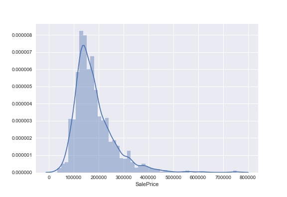
This figure describes the distribution of target variable. It does not look like a normal distribution and seems to have heavy tail.
print(y.skew())
print(y.kurt())
Skew and kurtosis of the distribution are 1.88 and 6.54 respectively.
from scipy import stats

stats.probplot(y, plot=plt, dist='norm', fit=True);
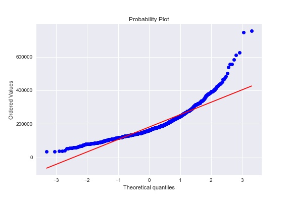
This figure is probaility plot. Considering skew, kurtosis, and probability plot, we conclude that the distribution is not nomral distribution. Let's try a transform of the target variable with log(x).
stats.probplot(np.log(y), plot=plt, dist='norm', fit=True);
print(np.log(y).skew())
print(np.log(y).kurt())
We did it!
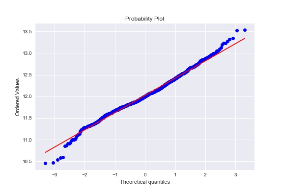
Given data seem to be on the line in the probability plot. Skew and kurtosis are 0.12 and 0.81 respectively. These facts imply that the target data spread with a normal distribution. In many cases, quadratic cost functions assume the gaussian noise, which gives you the normal distribution. Therefore, the transformed target variable is more convenient when working on optimization.
From now on, we use log(y) instead of y as a target variable.
df_train['SalePrice'] = np.log(df_train['SalePrice'])
3. Multivariate Analysis
While some features have significant effects on the behavior SalePrice, otheres do not. In this section, we work on figuring relations between variables.
Before working on analysis, we have to deal with missing data. Let's roll!
total = df_train.isnull().sum().sort_values(ascending=False)
total[:10].plot(kind='bar')
plt.title('The Number of Misssing Data')
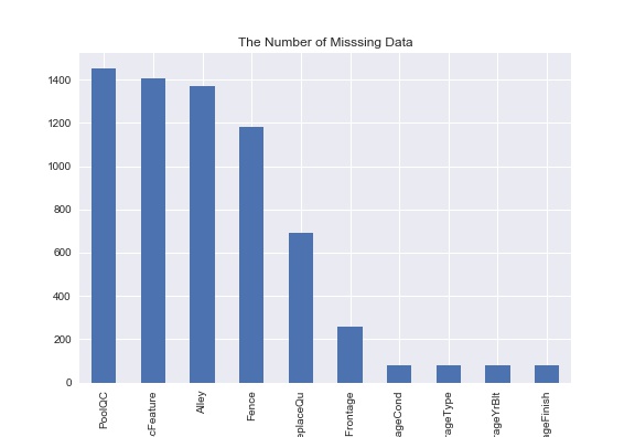
Most of candidates are missing top 3 features: PoolQC, MscFeature, and Alley. This may come from the fact that we do not care about these features when buying a house; e.g., we do not determine to purchase a house just because of the quality of pool (PoolQC).
For the sake of simplicity, we just treat these missing values as a new category 'MISSING' for category variables. For numerical variables, we use mean imputation.
from sklearn.preprocessing import Imputer

imp = Imputer()
for c in numerical:
    if df_train[c].isnull().any():
        df_train[c] = imp.fit_transform(df_train[c].values[:, np.newaxis])[:, 0]

for c in categorical:
    df_train[c] = df_train[c].astype('category')
    if df_train[c].isnull().any():
        df_train[c] = df_train[c].cat.add_categories(['MISSING'])
        df_train[c] = df_train[c].fillna('MISSING')
To analyze categorial variables along with numerical variables, we convert categorical variables into dummies.
yx_data = df_train[['SalePrice', ] + numerical + categorical]
yx_data = pd.get_dummies(yx_data)

corrmat = yx_data.corr()
f, ax = plt.subplots(figsize=(12, 12))
sns.heatmap(corrmat);
plt.title('Correlation Coefficient')
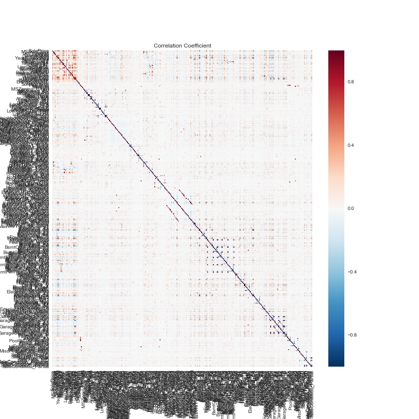
Oops! Too many columns! We consider reducing the number of features to a subset of features strongly correlated with the target variable.
We here use 20 features. We extract 20 features that have the largest abolute value of correlation coefficient with the target variable.
abs_corrmat = corrmat.copy()
abs_corrmat = abs_corrmat.set_value(
        index=corrmat.index,
        col=corrmat.columns,
        value=np.abs(corrmat.values)
    )
Let's pick up only higly correlated features.
large_cols = abs_corrmat.nlargest(20, 'SalePrice')['SalePrice'].index
large_corrmat = corrmat.loc[large_cols, large_cols]
f, ax = plt.subplots(figsize=(12, 12))
sns.heatmap(large_corrmat, square=True,
                       annot=True, cbar=True, fmt='.2f',
                       xticklabels=large_cols.values,
                       yticklabels=large_cols.values);
plt.title('Correlation Coefficient')
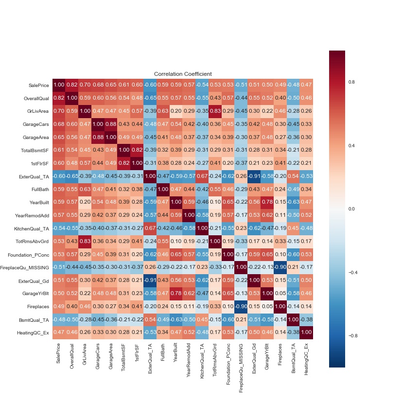
There are strong correlations in the following pairs: (GarageArea, GarageCars), (TotalBsmtSF, 1stFlrSF), (ExterQual_Gd, ExterQual_TA), (GarageYrBuilt, YearBuilt), and (TotRmsAbvTrd, GrLivArea). In the first pair, both express the size of garage. The second one describes the area of basement and first floor. The third one is separated just because of introducing dummy. Both elements in the fourth one explain how old. In the last one, each element expresses living area and total rooms. In any of the above five pairs, it is natural that two elements are correlated to each other within each pair. Therefore, it is good enough to use either of two elements for each pair.
remove_cols = ['GarageCars', '1stFlrSF', 'ExterQual_TA',
                            'GrLivArea', 'GarageYrBlt']
for x in remove_cols:
    large_cols = large_cols.drop(x)

large_corrmat = corrmat.loc[large_cols, large_cols]
f, ax = plt.subplots(figsize=(12, 12))
sns.heatmap(large_corrmat, square=True,
                       annot=True, cbar=True, fmt='.2f',
                       xticklabels=large_cols.values,
                       yticklabels=large_cols.values);
plt.title('Correlation Coefficient')

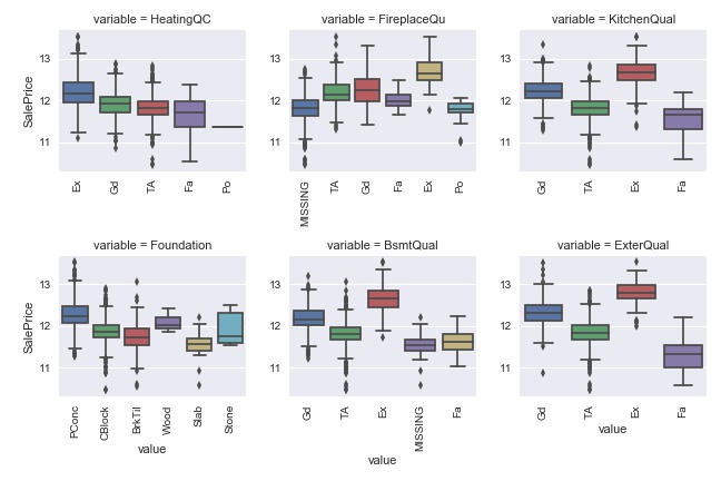
Let's see more precise relations between the target variable and selected features.
# extract only feature name and avoid duplication
large_cat = list(set([x.split('_')[0] for x in large_cols.values if '_' in x]))
large_num = [x.split('_')[0] for x in large_cols.values if '_' not in x]
# make figures for YearBuilt and OverallQual seperately
large_num.remove('OverallQual')
large_num.remove('YearBuilt')
f, ax = plt.subplots(figsize=(12, 6))
sns.boxplot(x=df_train['OverallQual'], y=df_train['SalePrice']);
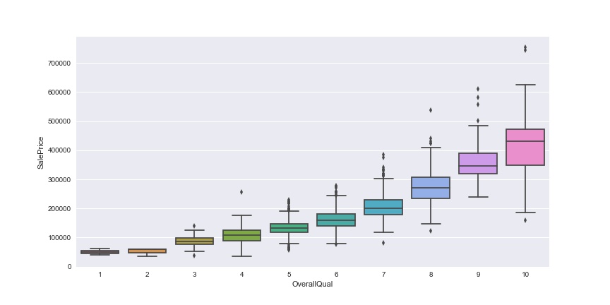
As we expected, the more OverallQual, the higher SalePrice.
f, ax = plt.subplots(figsize=(12,  6))
sns.boxplot(x=df_train['YearBuilt'], y=df_train['SalePrice']);
plt.xticks(rotation=90)
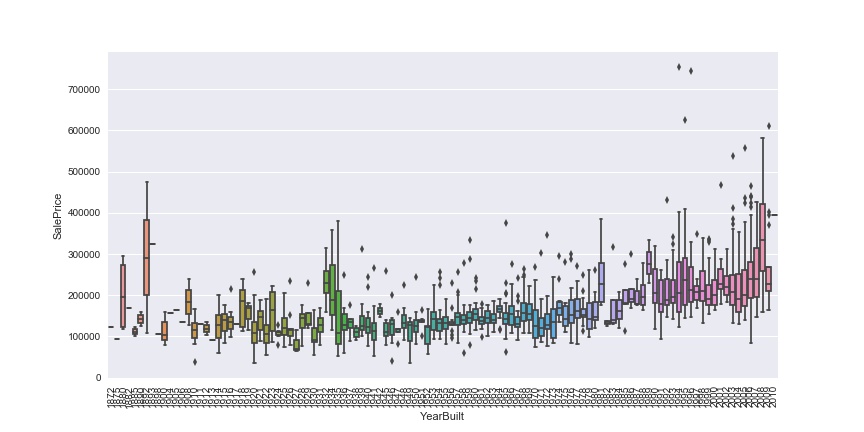
There seems to be a tendency that newer houses have higher prices. Let's see the effects of other categorical variables on the target variable.
melted_train = pd.melt(df_train, id_vars=['SalePrice'], value_vars=large_cat)

def boxplot(x, y, **kwargs):
    sns.boxplot(x=x, y=y)
    plt.xticks(rotation=90);

g = sns.FacetGrid(melted_train, col='variable', col_wrap=3,
                               sharex=False, sharey=False)
g.map(boxplot, 'value', 'SalePrice')
sns.pairplot(df_train[large_num], size=1.5);
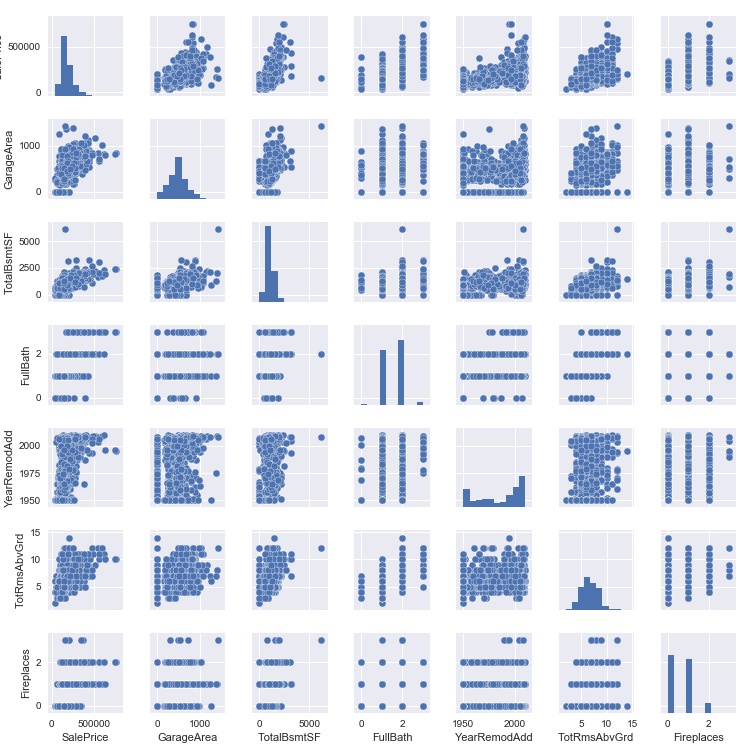
Look at the top raw. Generally speaking, the larger value feature tend to have higer prices.
4. Feature Selection
So far, we have been analyzing the relation through correlation coefficient and visualization. Random forest work as an alternative method to figure out the relations. Indeed, random forest is one of the most popular methods to select important features.
from sklearn.ensemble import RandomForestRegressor

X_full = yx_data[yx_data.columns.drop('SalePrice')]
y, X = df_train['SalePrice'].values[:, np.newaxis], X_full.values
clf = RandomForestRegressor(n_estimators=100)
clf.fit(X, y)

importance = clf.feature_importances_
argidx = np.argsort(importance)[::-1]
df_importance = pd.DataFrame(importance[argidx[:20]],
                                                       index=yx_data.columns.values[argidx[:20]])
imp_cols = yx_data.columns.values[argidx][:20]
df_importance.plot(kind='bar');
plt.title('Feature Importance')
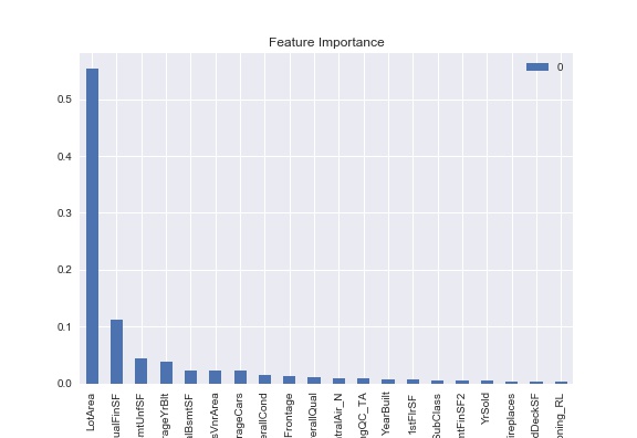
This figure describes the 20 features with the largest feature of importance.
Features selected Through correlation coefficient are
'LotArea', 'LowQualFinSF', 'BsmtUnfSF', 'GarageCars', 'GarageYrBlt', 'MasVnrArea', 'TotalBsmtSF', 'OverallCond', 'HeatingQC_TA', 'OverallQual', 'CentralAir_N', 'LotFrontage', '1stFlrSF', 'YearBuilt', 'BsmtFinSF2', 'GarageType_CarPort', 'MSSubClass', 'TotRmsAbvGrd', 'MSZoning_RL', 'WoodDeckSF'
In the feature of importance, selected features are
'SalePrice', 'OverallQual', 'GrLivArea', 'GarageCars', 'GarageArea', 'TotalBsmtSF', '1stFlrSF', 'ExterQual_TA', 'FullBath', 'YearBuilt', 'YearRemodAdd', 'KitchenQual_TA', 'TotRmsAbvGrd', 'Foundation_PConc', 'FireplaceQu_MISSING', 'ExterQual_Gd', 'GarageYrBlt', 'Fireplaces', 'BsmtQual_TA', 'HeatingQC_Ex'
They share the following features:
'1stFlrSF', 'GarageCars', 'GarageYrBlt', 'OverallQual', 'TotRmsAbvGrd', 'TotalBsmtSF', 'YearBuilt'
0nly 7 features are shared. Besides that, the feature with the largest importance, 'LotArea' is not even selected as top 20 through correlation coefficient. Let's compare the performances through linear regression.
def error(y, y_pred):
    return np.mean((y - y_pred)**2)
from sklearn.linear_model import LinearRegression
from sklearn.model_selection import KFold

kf = KFold(5)

y, X =yx_data['SalePrice'], yx_data[large_cols]

error_lr = []
for train, test in kf.split(X.values):
    X_train, X_test = X.values[train], X.values[test]
    y_train, y_test = y.values[train], y.values[test]
    lr = LinearRegression()
    lr.fit(X_train, y_train[:, np.newaxis])
    y_pred = lr.predict(X_test)[:, 0]
    error_lr.append(error(y_test, y_pred))
error_lr = np.mean(error_lr)

y, X =yx_data['SalePrice'], yx_data[imp_cols]

error_rf = []
for train, test in kf.split(X.values):
    X_train, X_test = X.values[train], X.values[test]
    y_train, y_test = y.values[train], y.values[test]
    lr = LinearRegression()
    lr.fit(X_train, y_train)
    y_pred = lr.predict(X_test)
    error_rf.append(error(y_test, y_pred))
error_rf = np.mean(error_rf)

index = np.arange(len(yx_data.columns))
np.random.shuffle(index)
random_cols = yx_data.columns[index[:20]]
y, X =yx_data['SalePrice'], yx_data[random_cols]

error_random = []
for train, test in kf.split(X.values):
    X_train, X_test = X.values[train], X.values[test]
    y_train, y_test = y.values[train], y.values[test]
    lr = LinearRegression()
    lr.fit(X_train, y_train)
    y_pred = lr.predict(X_test)
    error_random.append(error(y_test, y_pred))
error_random = np.mean(error_random)
| Method | Error |
|---|---|
| Correlation Coefficient | 0.0299 |
| Random Forest | 0.0300 |
| Random | 0.0935 |
Above figure is the cross validation of squared error with 20 features chosen by the following methods: correlation coefficient, random forest, and random. The first two methods have been discussed so far. Random means here choosing 20 features at random. First two methods have way better results than the random one.