Bayesian Optimization of Hyperparameters with Python

March 11, 2018

tags:
AutoML

Choosing a good set of hyperparameters is one of most important steps, but it is annoying and time consuming. The small number of hyperparameters may allow you to find an optimal set of hyperparameters after a few trials. This is, however, not the case for complex models like neural network.

When I just started my career as a data scientist, I was always frustrated to tune hyperparameters of Neural Network not to either underfit or overfit.

frustration

Actually there were a lot of ways to tune parameters efficiently and algorithmically, which I was ignorant of back in those days. Especially how to tune Neural Network has been progress rapidly in a recent few years by utilizing various algorithms: spectral analysis [1], bandit algorithms [2], evolutionary strategy [3], reinforcement learning [4], etc. How to build predictive general models algorithmically is also one of the hot research topics. Many frameworks and algorithms have been suggested [5], [6].

Some of algorithms are successful in outperforming state-of-art manually tuned models. Thus, building solid tuning algorithms could be cheaper and more efficient than hiring data scientists for tuning models.

scientist

In this blog post, we will go through the most basic three algorithms: grid, random, and Bayesian search. And, we will learn how to implement it in python.

Background

When optimizing hyperparameters, information available is score value of defined metrics(e.g., accuracy for classification) with each set of hyperparameters. We query a set of hyperparameters and get a score value as a response. Thus, optimization algorithms have to make efficient queries and find an optimal set without knowing how objective function looks like. This kind of optimization problem is called balck-box optimization. Here is the definition of black-box optimization:

"Black Box" optimization refers to a problem setup in which an optimization algorithm is supposed to optimize (e.g., minimize) an objective function through a so-called black-box interface: the algorithm may query the value f(x) for a point x, but it does not obtain gradient information, and in particular it cannot make any assumptions on the analytic form of f (e.g., being linear or quadratic). We think of such an objective function as being wrapped in a black-box. The goal of optimization is to find an as good as possible value f(x) within a predefined time, often defined by the number of available queries to the black box. Problems of this type regularly appear in practice, e.g., when optimizing parameters of a model that is either in fact hidden in a black box (e.g., a third party software library) or just too complex to be modeled explicitly.

by Balck-Box Optimization Competition homepage.

* There are some hyperparameter optimization methods to make use of gradient information, e.g., [7].

Grid, random, and Bayesian search, are three of basic algorithms of black-box optimization. They have the following characteristics (We assume the problem is minimization here):

Grid Search

Grid search is the simplest method. First, we place finite number of points on each hyperparameter axis and then make grid points by combining them. Here is the example:

A: (1e-8, 1e-6, 1e-4)
B: (0, 1)
(A, B): [(1e-8, 0), (1e-8, 1), (1e-6, 0) (1e-6, 1) (1e-4, 0) (1e-4, 1)]

When you have only a few hyperparameters, this method may works. Once dimension increases, the number of trials blows up exponentially.

Random Search

Random search is known effective over high dimensional search space. Especially when we have small subsets of effective hyperparameters out of high dimensional space, we search these effective parameters effectively [8].

Bayesian Search

While random search samples points independently, Bayesian search samples promising points more effectively by utilizing historical results. We first use GP (Gaussian process) to estimate objective function based on historical results [9].

GP also outputs variance along with mean. If this variance is large, small mean does not necessary imply promising because high values also likely happen as well. Points minimizing mean of estimation function are not necessary optimal. Thus, we need to define metric to consider trade off between mean and variance.

We introduce functions called acquisition function to deal with this issue. One of the most commonly used function is Expected Improvement. Here is the definition:

$$a_{EI}(x; \{x_n, y_n\}, \theta) = E[max(f(x_{best}) - f(x), 0) | \{x_n, y_n\}, \theta]$$

where $f(\cdot)$ is score function; $\{x_n, y_n\}$ historical input and its response from score function; $\theta$ is parameters of Gaussian process; $E[\cdot]$ is taking expectation with respect to a Gaussian probability.

The right hand can be calculated analytically to the following form:

$$a_{EI}(x; \{x_n, y_n\}, \theta) = \sigma(x ; \{x_n, y_n\}, \theta) [\gamma(x) \Phi(\gamma(x)) + N (\gamma(x); 0, 1)]$$

where

$$\gamma(x) = \frac{f(x_{best}) − \mu(x ; \{x_n, y_n\}, \theta)}{\sigma(x ; \{x_n, y_n\}, \theta)}$$

$N(\cdot; 0, 1)$ and $\Phi(\cdot)$ are p.d.f. and c.d.f of Gaussian distribution, respectively.

Here is python code:

import numpy as np

def expected_improvement(x, model, evaluated_loss, jitter=0.01):
    """ expected_improvement
    Expected improvement acquisition function.

    Note
    ----
    This implementation aims for minimization

    Parameters:
    ----------
    x: array-like, shape = (n_hyperparams,)
    model: GPRegressor object of GPy.
        Gaussian process trained on previously evaluated hyperparameters.
    evaluated_loss: array-like(float), shape = (# historical results,).
         the values of the loss function for the previously evaluated
         hyperparameters.
    jitter: float
        positive value to make the acquisition more explorative.
    """
    x = np.atleast_2d(x)
    mu, var = model.predict(x)
    # Consider 1d case
    sigma = np.sqrt(var)[0, 0]
    mu = mu[0, 0]
    # Avoid too small sigma
    if sigma == 0.:
        return 0.
    else:
        loss_optimum = np.min(evaluated_loss)
        gamma = (loss_optimum - mu - jitter) / sigma
        ei_val = sigma * (gamma * norm.cdf(gamma) + norm.pdf(gamma))
        return ei_val

Summing up the above discussion, Bayesian optimization is executed in the following steps: 1. Sample a few points and score them. 2. Initialize GP with sampled points 3. Sample points that minimize acquisition function 4. Score sampled points and store the results in GP 5. Iterate 3. and 4.

To implement them in python, I have implemented two class objects: Sampler and Optimizer.

Sampler class basically consists of two methods: - update: Update GP based on historical results - sample: Sample optimal points with respect to an acquisition function

Optimizer class utilizes a sampler to find optimal points.

Here are python codes for the step 3. and 4.:

Step 3.

def _bayes_sample(self, num_restarts=25):
    init_xs = self._random_sample(num_restarts)
    # Define search space
    bounds = self.design_space.get_bounds()
    # Historical results
    evaluated_loss = self._y
    ys = []
    xs = []

    # Find a point to minimize acquisition function
    for x0 in init_xs:
        res = minimize(fun=-self.acquisition_func,
                       x0=x0,
                       bounds=bounds,
                       method='L-BFGS-B',
                       args=(self.model, evaluated_loss))
        ys.append(-res.fun)
        xs.append(res.x)
    idx = np.argmax(ys)
    best_x = np.array(xs)[idx]
    return best_x

def _random_sample(self, num_samples):
    Xs = []
    for i in range(num_samples):
        x = random_sample(self.params_conf)
        Xs.append(x)
    return list(Xs)

Step 4.

def _update(self, eps=1e-6):
    X, y = self.data
    y = np.array(y)[:, None]
    # Update data in GP
    self.model.set_XY(X_vec, y)
    # Update hyperparameters of GP
    self.model.optimize()

self.model.optimize() optimize GP model defined at GPy. Then, we use these update and sample methods of the sampler object to optimize parameters

for i in range(num_iter):
    Xs = sampler.sample(*args, **kwargs)
    ys = []
    for X in Xs:
        y = self.score_func(X)
        ys.append(y)
        sampler.update(Xs, ys)
    Xs, ys = sampler.data
    best_idx = np.argmin(ys)
    # Default is minimization
    if self._maximize:
        ys = -ys
    # Update with  fixed parameters
    best_X = Xs[best_idx]
    best_y = ys[best_idx]
    return best_X, best_y

To make it easy to understand the above codes, I change some parts from actual implementation. If you want to see the full implementation, check out this repository.

Experiments

Let's compare performance of these algorithms!!

Toy Model

As a simple example, we shall test the following function:

import numpy as np

map_func = dict(linear=lambda x: x, square=lambda x: x**2, sin=np.sin)

def score_func(x):
    score = np.sin(x["x2"]) + map_func[x["x4"]](x["x1"]) + map_func[x["x4"]](x["x3"])
    score_val = -score
    return score_val


params_conf = [
    {"name": "x1", "domain": (.1, 5), "type": "continuous",
     "num_grid": 5, "scale": "log"},
    {"name": "x2", "domain": (-5, 3), "type": "continuous",
     "num_grid": 5},
    {"name": "x3", "domain": (-3, 5), "type": "continuous",
     "num_grid": 5},
    {"name": "x4", "domain": ("linear", "sin", "square"),
     "type": "categorical"},
]

The x3 determines which function is used with for the two variables: x1 and x3. Comparatively speaking, x2 does not affect the performance because of sine function. The precise way of defining search space is explained in my repository.

From the definition above, we know the optimal result in advance:

params = {'x1': 5, 'x2': 3.141592..., 'x3', 5.0, 'x4': 'sqaure'}
score = 51.0

To execute optimization, we use

import random
import numpy as np
from bboptimizer import Optimizer

np.random.seed(0)
random.seed(0)
bayes_opt = Optimizer(score_func, params_conf, sampler="bayes", r_min=10, maximize=True)
bayes_opt.search(num_iter=50)


np.random.seed(0)
random.seed(0)
random_opt = Optimizer(score_func, params_conf, sampler="random", maximize=True)
random_opt.search(num_iter=50)


np.random.seed(0)
random.seed(0)
grid_opt = Optimizer(score_func, params_conf, sampler="grid", num_grid=3, maximize=True)
grid_opt.search(num_iter=50)

Here is the result:

toy_model_opt

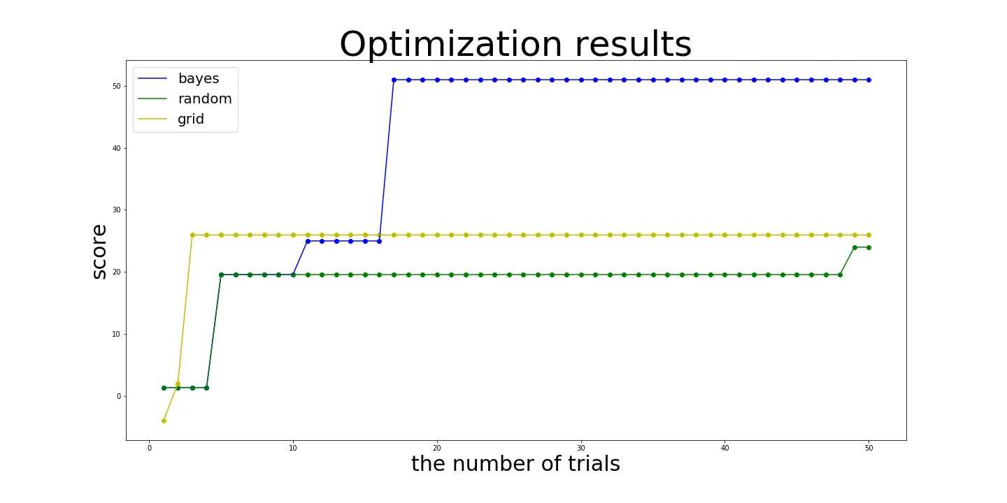
In this example, Bayesian search achieves the almost optimal values:

best_parmas = {'x1': 5, 'x2': -5.0, 'x3': -5.0, 'x4': 'square'}
best_score = 50.95892427466314

after 8 Bayesian samples and 10 random initialization while random and grid search achieve 24.004995120648054 and 25.968924274663138 even after 50 trials. In this example, grid search works slightly better than random search. This is because optimal values of x2 and x3 are placed at the end of search space, which allows grid search to try these values deterministically.

Hyperparameter Optimization

Next problem is tuning hyperparameters of one of the basic machine learning models, Support Vector Machine. We consider optimizing regularization parameters C and gamma with accuracy score under fixed kernel to RBF at scikit-learn implementation. We use an artificially classification problem made up with make_classification of scikit-learn. Let's set up the problem!

from sklearn.svm import SVC
from sklearn.datasets import make_classification
from sklearn.metrics import accuracy_score
from sklearn.model_selection import StratifiedShuffleSplit


data, target = make_classification(n_samples=2500,
                                   n_features=45,
                                   n_informative=5,
                                   n_redundant=5)


def score_func(params):
    splitter = StratifiedShuffleSplit(n_splits=1, test_size=0.2)
    train_idx, test_idx = list(splitter.split(data, target))[0]
    train_data = data[train_idx]
    train_target = target[train_idx]
    clf = SVC(**params)
    clf.fit(train_data, train_target)
    pred = clf.predict(data[test_idx])
    true_y = target[test_idx]
    score = accuracy_score(true_y, pred)
    return score

params_conf = [
    {'name': 'C', 'domain': (1e-8, 1e5), 'type': 'continuous', 'scale': 'log'},
    {'name': 'gamma', 'domain': (1e-8, 1e5), 'type': 'continuous', 'scale': 'log'},
    {'name': 'kernel', 'domain': 'rbf', 'type': 'fixed'}
]

Here is the results:

hyper_opt

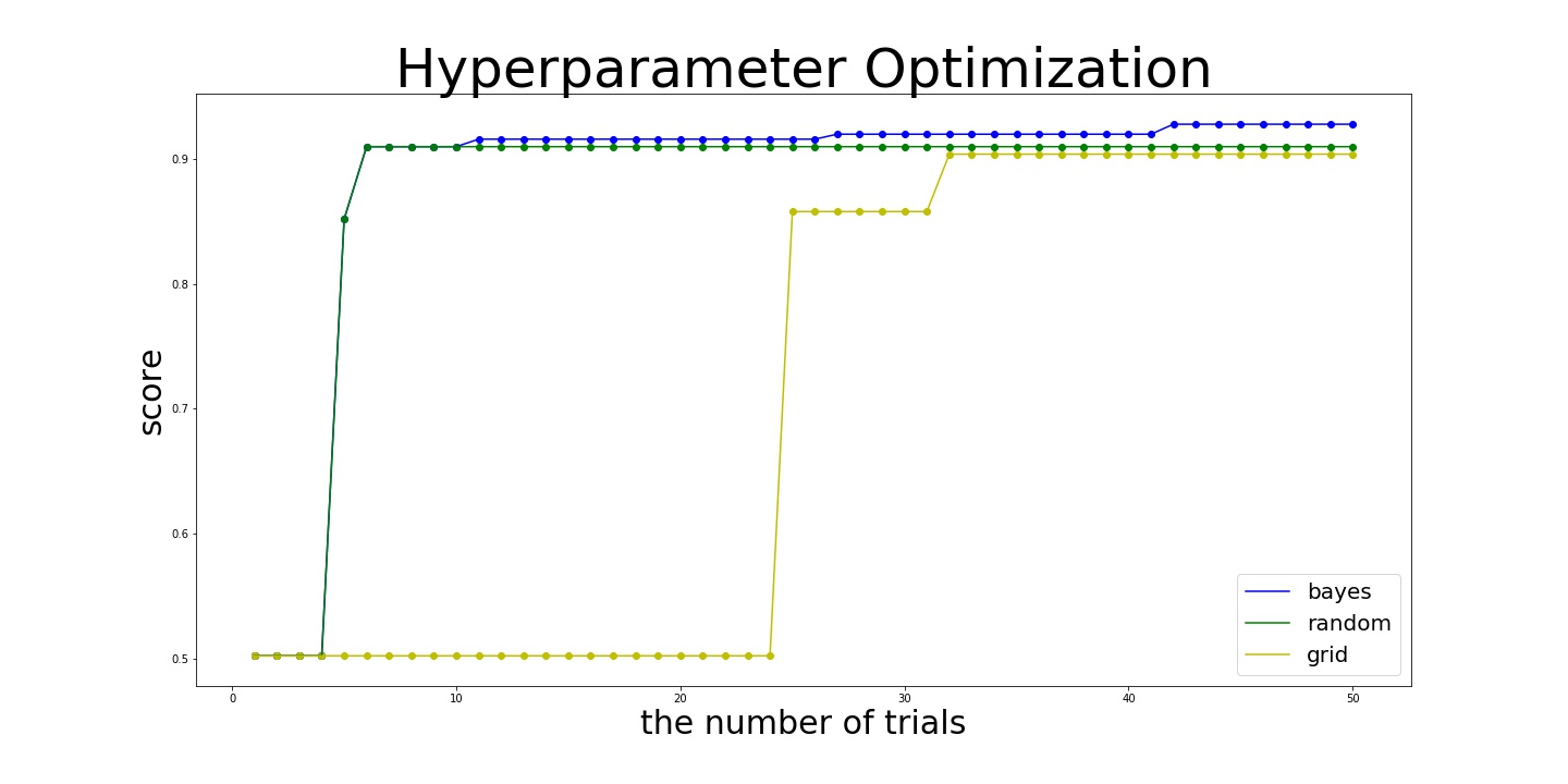
bayes

best_params={'C': 100000.0, 'gamma': 0.03836608377440943, 'kernel': 'rbf'}
best_score=0.928

random:

best_params={'C': 196.07647697179934, 'gamma': 0.07509896588333721, 'kernel': 'rbf'}
best_score= 0.91

grid:

best_params={'C': 4.641588833612772, 'gamma': 0.03162277660168379, 'kernel': 'rbf'}
best_score=0.904

As you see in the result above, Bayesian optimization outperformed other algorithms.

Hyperparameters Optimization Neural Network

As a final example, we are going to optimize hyperparameters of Neural Network. For the sake of the simplicity, we define hyperparameters with the following parameters:

For training configuration, we define - learning rate - the number of training epochs - optimization algorithm - batch size

For each input, hidden, output layers we define - the number of layers - the number of hidden units - weight regularizer - activation function - dropout rate - if use batch normalization

Thus, we have 22 hyperparameters, which is almost infeasible to be optimized by grid search. In this example, we test Bayesian and random search to find good set of 22 hyperparameters.

To test optimization algorithms, we use machine learning "hello world" problem, classifying MNIST handwrite digit data. We fetch data from tensorflow interface and use the train and valid data.

Let's set up the problem:

from sklearn.preprocessing import OneHotEncoder
import numpy as np
import tensorflow as tf
from keras.models import Sequential
from keras.layers import Dense, BatchNormalization, Dropout
from keras.layers import Activation, Reshape
from keras.optimizers import Adam, Adadelta, SGD, RMSprop
from keras.regularizers import l2

from bboptimizer import Optimizer

# Fetch MNIST dataset
mnist = tf.contrib.learn.datasets.load_dataset("mnist")


train = mnist.train
X = train.images
train_X = X
train_y = np.expand_dims(train.labels, -1)
train_y = OneHotEncoder().fit_transform(train_y)

valid = mnist.validation
X = valid.images
valid_X = X
valid_y = np.expand_dims(valid.labels, -1)
valid_y = OneHotEncoder().fit_transform(valid_y)


def get_optimzier(name, **kwargs):
    if name == "rmsprop":
        return RMSprop(**kwargs)
    elif name == "adam":
        return Adam(**kwargs)
    elif name == "sgd":
        return SGD(**kwargs)
    elif name == "adadelta":
        return Adadelta(**kwargs)
    else:
        raise ValueError(name)


def construct_NN(params):
    model = Sequential()
    model.add(Reshape((784,), input_shape=(784,)))

    def update_model(_model, _params, name):
        _model.add(Dropout(_params[name + "_drop_rate"]))
        _model.add(Dense(units=_params[name + "_num_units"],
                    activation=None,
                    kernel_regularizer=l2(_params[name + "_w_reg"])))
        if _params[name + "_is_batch"]:
            _model.add(BatchNormalization())
        if _params[name + "_activation"] is not None:
            _model.add(Activation(_params[name + "_activation"]))
        return _model

    # Add input layer
    model = update_model(model, params, "input")
    # Add hidden layer
    for i in range(params["num_hidden_layers"]):
        model = update_model(model, params, "hidden")
    # Add output layer
    model = update_model(model, params, "output")
    optimizer = get_optimzier(params["optimizer"],
                              lr=params["learning_rate"])
    model.compile(optimizer=optimizer,
              loss='categorical_crossentropy',
              metrics=['accuracy'])
    return model


def score_func(params):
    model = construct_NN(params)
    model.fit(train_X, train_y,
              epochs=params["epochs"],
              batch_size=params["batch_size"], verbose=1)
    score = model.evaluate(valid_X, valid_y,
                  batch_size=params["batch_size"])
    idx = model.metrics_names.index("acc")
    score = score[idx]
    print(params, score)
    return score

params_conf = [
    {"name": "num_hidden_layers", "type": "integer",
     "domain": (0, 5)},
    {"name": "batch_size", "type": "integer",
     "domain": (16, 128), "scale": "log"},
    {"name": "learning_rate", "type": "continuous",
     "domain": (1e-5, 1e-1), "scale": "log"},
    {"name": "epochs", "type": "integer",
     "domain": (10, 250), "scale": "log"},
    {"name": "optimizer", "type": "categorical",
     "domain": ("rmsprop", "sgd", "adam", "adadelta")},

    {"name": "input_drop_rate", "type": "continuous",
     "domain": (0, 0.5)},
    {"name": "input_num_units", "type": "integer",
     "domain": (32, 512), "scale": "log"},
    {"name": "input_w_reg", "type": "continuous",
     "domain": (1e-10, 1e-1), "scale": "log"},
    {"name": "input_is_batch", "type": "categorical",
     "domain": (True, False)},
    {"name": "input_activation", "type": "categorical",
     "domain": ("relu", "sigmoid", "tanh")},

    {"name": "hidden_drop_rate", "type": "continuous",
     "domain": (0, 0.75)},
    {"name": "hidden_num_units", "type": "integer",
     "domain": (32, 512), "scale": "log"},
    {"name": "hidden_w_reg", "type": "continuous",
     "domain": (1e-10, 1e-1), "scale": "log"},
    {"name": "hidden_is_batch", "type": "categorical",
     "domain": (True, False)},
    {"name": "hidden_activation", "type": "categorical",
     "domain": ("relu", "sigmoid", "tanh")},

    {"name": "output_drop_rate", "type": "continuous",
     "domain": (0, 0.5)},
    {"name": "output_num_units", "type": "fixed",
     "domain": 10},
    {"name": "output_w_reg", "type": "continuous",
     "domain": (1e-10, 1e-1), "scale": "log"},
    {"name": "output_is_batch", "type": "categorical",
     "domain": (True, False)},
    {"name": "output_activation", "type": "fixed",
     "domain": "softmax"},

]

Here is the result:

hyper_opt

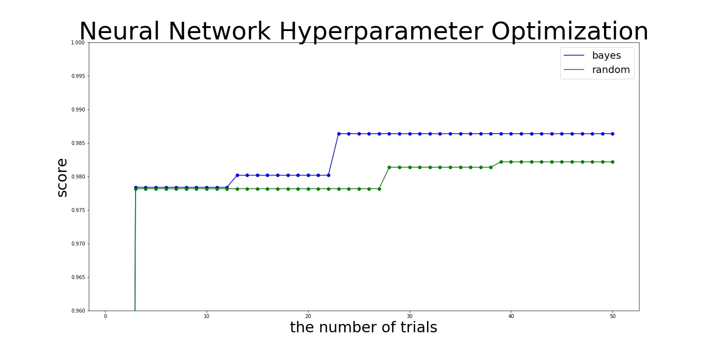
bayes:
best_params = {'num_hidden_layers': 0,
               'batch_size': 128,
               'learning_rate': 0.0009053002734681439,
               'epochs': 250,
               'optimizer': 'rmsprop',
               'input_drop_rate': 0.5,
               'input_num_units': 512,
               'input_w_reg': 1.2840834618450513e-06,
               'input_is_batch': True,
               'input_activation': 'sigmoid',
               'hidden_drop_rate': 0.0,
               'hidden_num_units': 41,
               'hidden_w_reg': 6.970606129393136e-07,
               'hidden_is_batch': True,
               'hidden_activation': 'relu',
               'output_drop_rate': 0.0,
               'output_w_reg': 1e-10,
               'output_is_batch': True,
               'output_num_units': 10,
               'output_activation': 'softmax'}

best_score = 0.9864


random:
best_params = {'batch_size': 74,
               'epochs': 204,
               'hidden_activation': 'tanh',
               'hidden_drop_rate': 0.6728025784523577,
               'hidden_is_batch': False,
               'hidden_num_units': 45,
               'hidden_w_reg': 1.4924891356983298e-08,
               'input_activation': 'relu',
               'input_drop_rate': 0.12861674273569668,
               'input_is_batch': True,
               'input_num_units': 92,
               'input_w_reg': 0.00018805052553280536,
               'learning_rate': 0.0006256532585348427,
               'num_hidden_layers': 0,
               'optimizer': 'adam',
               'output_activation': 'softmax',
               'output_drop_rate': 0.11413180495018566,
               'output_is_batch': False,
               'output_num_units': 10,
               'output_w_reg': 2.544391637336686e-06}

best_score = 0.9822000049591064

In this example, Bayesian search finds that maximum value of the number of epochs is more likely to bring better score and keep using this value from the middle of searching. Then, Bayesian search finds better values more efficiently.

Wrap Up

As we go through in this article, Bayesian optimization is easy to implement and efficient to optimize hyperparameters of Machine Learning algorithms. If you have computer resources, I highly recommend you to parallelize processes to speed up [10]. As you have time, you can also try to use Bayesian methods to utilize gradient information [11].

Background

Grid Search

Random Search

Bayesian Search

Experiments

Toy Model

Hyperparameter Optimization

Hyperparameters Optimization Neural Network

Wrap Up

References